Introduction
Suppose $\chi_{l,m}(\mathbf{r})$ is a atomic orbital of the form:
\[\begin{equation} \chi_{l,m}(\mathbf{r}) = f_{l}(r)\cdot Y_l^m(\hat{\mathbf{r}}) \end{equation}\]where $f_l(r)$ is the radial part and $Y_l^m$ is the complex spherical harmonics. 1 Two types of functions are often used as atomic orbitals, i.e. Slater-type orbital (STO) 2
\[\begin{equation} f_{n,l}^{\text{STO}}(r) = (2\zeta)^{n+\frac{1}{2}}[(2n)!]^{-\frac{1}{2}}\, r^{n-1}e^{-\zeta r} \end{equation}\]and Gaussian-type orbital (GTO): 3
\[\begin{equation} f_{n,l}^{\text{GTO}}(r) = B(l,\alpha)\, r^l e^{-\alpha r^2} \end{equation}\]The Fourier transform of $\chi_{l,m}(\mathbf{r})$ is a function of the same form, i.e. 4
\[\begin{equation} \tilde\chi_{l,m}(\mathbf{k}) = \int \chi_{l,m}(\mathbf{r})\,e^{-i\mathbf{k}\cdot\mathbf{r}} \,\mathrm{d}\mathbf{r} = i^{-l}\,g_{l}(k)\cdot Y_l^m(\hat{\mathbf{k}}) \end{equation}\]where $g_l(k)$ is the spherical Bessel transform (SBT) of $f_l(r)$.
\[\begin{equation} g_l(k) = \sqrt{\frac{2}{\pi}} \int_0^\infty j_l(kr)f_l(r)r^2 \mathrm{d} r \end{equation}\]Let us consider first the overlap integral (or $S$-matrix) of two atomic orbitals with a distance $\mathbf{R}$
\[\begin{equation} S(R) = \braket{\chi_{l_1,m_1}(\mathbf{r}) | \chi_{l_2,m_2}(\mathbf{r} - \mathbf{R})} \label{eq:s_def} \end{equation}\]The integral can be performed in real-space, i.e.
\[\begin{equation} S(R) = \int \chi^*_{l_1,m_1}(\mathbf{r})\, \chi_{l_2,m_2}(\mathbf{r} - \mathbf{R}) \mathrm{d}\mathbf{r} \label{eq:s_def_r} \end{equation}\]or momentum space (Fourier space):
\[\begin{equation} S(R) = \int \tilde\chi^*_{l_1,m_1}(\mathbf{k})\, \tilde\chi_{l_2,m_2}(\mathbf{k}) e^{-i\mathbf{k}\cdot\mathbf{R}} \mathrm{d}\mathbf{k} \label{eq:s_def_k} \end{equation}\]where the phase $e^{-i\mathbf{k}\cdot\mathbf{R}}$ in Eq.\eqref{eq:s_def_k} is due to the shifting property of Fourier trasnform.
Overlap integral in momentum space
Starting with Eq.\eqref{eq:s_def_k} and remember that the plane-wave can be expanded by spherical waves, i.e. 4
\[\begin{equation} \label{eq:pw_exp} e^{-i\mathbf{k}\cdot\mathbf{R}} = 4\pi\sum_{l=0}^\infty \sum_{m=-l}^l i^{-l} \,j_l(kR) \, Y_l^{m*}(\hat{\mathbf{k}}) \, Y_l^{m}(\hat{\mathbf{R}}) \end{equation}\]where $Y_l^m(\theta, \phi)$ are the complex spherical harmonics. Inserting Eq.\eqref{eq:pw_exp} into Eq.\eqref{eq:s_def_k}, one can have
\[\begin{align} S(\mathbf{R}) &= 4\pi \sum_{l=0}^\infty \sum_{m=-l}^l i^{l_1 - l_2 - l} \int g_{l_1}(k) Y_{l_1}^{m_1*}(\hat{\mathbf{k}}) \, g_{l_2}(k) Y_{l_2}^{m_2}(\hat{\mathbf{k}}) \,\, j_l(kR) Y_{l}^{m*}(\hat{\mathbf{k}}) Y_{l}^{m}(\hat{\mathbf{R}}) \, k^2 \mathrm{d}k \mathrm{d}\Omega \label{eq:s_final_1} \\ &= 4\pi \sum_{l=0}^\infty \sum_{m=-l}^l i^{l_1 - l_2 - l} (-1)^{m_1 + m} {\cal G}(l_1, l_2, l, \mbox{-}m_1, m_2, \mbox{-}m) Y_l^m(\hat{\mathbf{R}}) \int_0^\infty\!\!\! g_{l_1}(k) \, g_{l_2}(k) \, j_l(kR) k^2 \mathrm{d}k \label{eq:s_final} \end{align}\]where ${\cal G}$ is the Gaunt coefficient defined as integral over three complex spherical harmonics
\[\begin{equation} \label{eq:gaunt_complex_sph} {\cal G}(l_1, l_2, l_3, m_1, m_2, m_3) = \int_{\theta=0}^{\pi}\int_{\phi=0}^{2\pi} Y_{l_1}^{m_1}(\theta, \phi) \, Y_{l_2}^{m_2}(\theta, \phi) \, Y_{l}^{m}(\theta, \phi) \, \sin\theta\mathrm{d}\theta \mathrm{d}\phi \end{equation}\]-
Note that $Y_l^{m*}(\theta, \phi) = (-1)^m Y_l^{-m}(\theta, \phi)$ is used from Eq.\eqref{eq:s_final_1} to Eq.\eqref{eq:s_final}.
-
The integral over $k$ in Eq.\eqref{eq:s_final} is the inverse spherical Bessel transform of $g_{l_1}(k)\, g_{l_2}(k)$.
-
In practice, real spherical harmonics $Y_{l,m}(\theta, \phi)$ are often used, which does not affect the validity of any of previous equations, but the Gaunt coefficients should be modified accordingly.
\[\begin{equation} \label{eq:s_final_realsph} S(\mathbf{R}) = 4\pi \sum_{l=0}^\infty \sum_{m=-l}^l i^{l_1 - l_2 - l} {\cal G}'(l_1, l_2, l, m_1, m_2, m) Y_{l,m}(\hat{\mathbf{R}}) \int_0^\infty g_{l_1}(k) g_{l_2}(k) j_l(kR) \, k^2 \mathrm{d}k \end{equation}\]and
\[\begin{equation} \label{eq:gaunt_real_sph} {\cal G}'(l_1, l_2, l_3, m_1, m_2, m_3) = \int_{\theta=0}^{\pi}\int_{\phi=0}^{2\pi} Y_{l_1,m_1}(\theta, \phi) \, Y_{l_2,m_2}(\theta, \phi) \, Y_{l,m}(\theta, \phi) \, \sin\theta\mathrm{d}\theta \mathrm{d}\phi \end{equation}\]
Gaunt coefficients
Complex spherical harmonics
They Gaunt coefficients defined as Eq.\eqref{eq:gaunt_complex_sph} are related to Wigner-$3j$ symbol by 5
\[\begin{equation} \label{eq:gaunt_wigner3j} {\cal G}(l_1, l_2, l_3, m_1, m_2, m_3) = \sqrt{\frac{(2l_1+1)(2l_2+1)(2l_3+1)}{4\pi}} \begin{pmatrix} l_1 & l_2 & l_3 \\ 0 & 0 & 0 \end{pmatrix} \begin{pmatrix} l_1 & l_2 & l_3 \\ m_1 & m_2 & m_3 \end{pmatrix} \end{equation}\]They obey the following symmetry rules
-
Invariant under space reflection, i.e.
\[\begin{equation} {\cal G}(l_1, l_2, l_3, m_1, m_2, m_3) = {\cal G}(l_1, l_2, l_3,-m_1,-m_2,-m_3) \end{equation}\] -
Invariant under any permutation of the columns, i.e.
\[\begin{equation} \begin{split} \begin{aligned} {\cal G}(l_1,l_2,l_3,m_1,m_2,m_3) &={\cal G}(l_3,l_1,l_2,m_3,m_1,m_2) ={\cal G}(l_2,l_3,l_1,m_2,m_3,m_1) \\ &={\cal G}(l_3,l_2,l_1,m_3,m_2,m_1) ={\cal G}(l_1,l_3,l_2,m_1,m_3,m_2) \\ &={\cal G}(l_2,l_1,l_3,m_2,m_1,m_3) \end{aligned} \end{split} \end{equation}\] -
Non-zero only for even sum of the $l_i$, i.e. $l_1 + l_2 + l_3 = 2n$ for $n \in \mathbb{N}$.
-
Non-zero for $l_1, l_2, l_3$ fulfilling the triangle relation, i.e. $|l_1 - l_2| \le l \le l_1 + l_2$.
-
Non-zero for $m_1 + m_2 + m_3 = 0$.
As a result, the sum in Eq.\eqref{eq:s_final} reduces to $\displaystyle \sum_{l=0}^\infty \sum_{m=-l}^l \Longrightarrow \sum_{l=|l_1-l_2|}^{l_1 + l_2} \sum_{m=-l}^l \delta_{m,m_2-m_1}$.
The Gaunt coefficients can be obtained by recursion from Clebsch–Gordan
coefficients.6 In sympy, one can get
1
2
3
4
from sympy.physics.wigner import gaunt
gaunt(0,0,0,0,0,0)                     # 1/(2*sqrt(pi))
gaunt(1,0,1,1,0,-1)                    # -1/(2*sqrt(pi))
gaunt(1000,1000,1200,9,3,-12).n(64)    # 0.00689500421922113448...
Real spherical harmonics
As is well known, complex and real spherical harmonics (SPH) can be inter-transformed by a unitary matrix $U^l$, i.e.7
\[\begin{equation} \label{eq:u_c2r} Y_{l,m}(\theta, \phi) = \sum_{n=0}^{2l+1} U^l_{m,n}Y_{l}^{n-l}(\theta, \phi) = \begin{cases} \frac{i}{\sqrt{2}}(Y_l^m - (-1)^m Y_l^{-m}) & \text{if } m < 0 \\ Y_l^0 & \text{if } m = 0 \\ \frac{1}{\sqrt{2}}(Y_l^{-|m|} + (-1)^m Y_l^m) & \text{if } m > 0 \end{cases} \end{equation}\]Therefore, the Gaunt coefficients defined in Eq.\eqref{eq:gaunt_real_sph} can then be written as
\[\begin{align} {\cal G}'(l_1, l_2, l_3, m_1, m_2, m_3) &= \int_{\theta=0}^{\pi}\int_{\phi=0}^{2\pi} Y_{l_1,m_1}(\theta, \phi) \, Y_{l_2,m_2}(\theta, \phi) \, Y_{l_3,m_3}(\theta, \phi) \, \sin\theta\mathrm{d}\theta \mathrm{d}\phi \\[6pt] &= \sum_{n_1=0}^{2l_1+1} \sum_{n_2=0}^{2l_2+1} \sum_{n_3=0}^{2l_3+1} U_{m_1,n_1}^{l_1} U_{m_2,n_2}^{l_2} U_{m_3,n_3}^{l_3} \,\, {\cal G}(l_1, l_2, l_3, n_1\mbox{-}l_1, n_2\mbox{-}l_2, n_3\mbox{-}l_3) \label{eq:real_gaunt_exp} \end{align}\]The Gaunt coefficients ${\cal G}’$ also obey the following rules
- Invariant under any permutation of the columns.
- Non-zero only for even sum of the $l_i$, i.e. $l_1 + l_2 + l_3 = 2n$ for $n \in \mathbb{N}$.
- Non-zero for $l_1, l_2, l_3$ fulfilling the triangle relation, i.e. $|l_1 - l_2| \le l \le l_1 + l_2$.
-
Zero for $m_1 < 0$, $m_2 < 0$ and $m_3 <0$. To see this, by combining Eq.\eqref{eq:u_c2r} and Eq.\eqref{eq:real_gaunt_exp}, we have
\[\begin{align*} {\cal G}'(l_1, l_2, l_3, m_1, m_2, m_3) &= \frac{-i}{2\sqrt{2}}\Bigl[\,{\cal G}(l_1, l_2, l_3, m_1, m_2, m_3) \\[3pt] &\quad{}-{} (-1)^{m_1+m_2+m_3}{\cal G}(l_1, l_2, l_3, \overline{m_1}, \overline{m_2}, \overline{m_3}) \\[6pt] &\quad{}+{} (-1)^{m_2+m_3}{\cal G}(l_1, l_2, l_3, {m_1}, \overline{m_2}, \overline{m_3}) \\[6pt] &\quad{}-{} (-1)^{m_1}{\cal G}(l_1, l_2, l_3, \overline{m_1}, {m_2}, {m_3}) \\[6pt] &\quad{}+{} (-1)^{m_1+m_3}{\cal G}(l_1, l_2, l_3, \overline{m_1}, {m_2}, \overline{m_3}) \\[6pt] &\quad{}-{} (-1)^{m_2}{\cal G}(l_1, l_2, l_3, {m_1}, \overline{m_2}, {m_3}) \\[6pt] &\quad{}+{} (-1)^{m_1+m_2}{\cal G}(l_1, l_2, l_3, \overline{m_1}, \overline{m_2}, {m_3}) \\[6pt] &\quad{}-{} (-1)^{m_3}{\cal G}(l_1, l_2, l_3, {m_1}, {m_2}, \overline{m_3})\Bigr] \end{align*}\]where we have used $\overline{m} = -m$ for abbreviation.
-
The Gaunt coefficients in the first two terms are apparently zero since all $m_i < 0$ and as a result the sum of $m_i$ could not possibly be zero.
-
For the Gaunt coefficients in the rest terms to be non-zero, one of the following conditions must be fulfilled:
\[\begin{equation} \label{eq:non-zero_cond} m_1 = m_2 + m_3;\quad m_2 = m_1 + m_3;\quad m_3 = m_1 + m_2 \end{equation}\]Let’s first assume that $m_1 = m_2 +m_3$ so that the Gaunt coefficients in the 3-rd and 4-th terms are not zero. Moreover, Due to the space reflection symmetry, the Gaunt coefficients in these two terms equal to each other. Apparently, the Gaunt coefficients in the rest terms are zero (we could not have $m_1 = m_2 + m_3$, $m_2 = m_1 + m_3$ and $m_3 = m_1 + m_2$ at the same time). Now the sign before the 3-rd and 4-th terms can be written as
\[\begin{equation} (-1)^{m_2 + m_3} - (-1)^{m_1} = (-1)^{m_1}[(-1)^{m_1 + m_2 + m_3} - 1] \end{equation}\]which is zero for $m_1 = m_2 +m_3$. The same reasoning applies to the 5/6 and 7/8 terms.
-
-
If $m_1 > 0$, $m_2 > 0$ and $m_3 >0$, then non-zero for $m_1 + m_2 + m_3 = 2n$ for $n\in\mathbb{N}$.
In this case, Eq.\eqref{eq:real_gaunt_exp} expands to
\[\begin{align*} {\cal G}'(l_1, l_2, l_3, m_1, m_2, m_3) &= \frac{1}{2\sqrt{2}}\Bigl[\,{\cal G}(l_1, l_2, l_3, m_1, m_2, m_3) \\[3pt] &\quad{}+{} (-1)^{m_1+m_2+m_3}{\cal G}(l_1, l_2, l_3, \overline{m_1}, \overline{m_2}, \overline{m_3}) \\[6pt] &\quad{}+{} (-1)^{m_2+m_3}{\cal G}(l_1, l_2, l_3, {m_1}, \overline{m_2}, \overline{m_3}) \\[6pt] &\quad{}+{} (-1)^{m_1}{\cal G}(l_1, l_2, l_3, \overline{m_1}, {m_2}, {m_3}) \\[6pt] &\quad{}+{} (-1)^{m_1+m_3}{\cal G}(l_1, l_2, l_3, \overline{m_1}, {m_2}, \overline{m_3}) \\[6pt] &\quad{}+{} (-1)^{m_2}{\cal G}(l_1, l_2, l_3, {m_1}, \overline{m_2}, {m_3}) \\[6pt] &\quad{}+{} (-1)^{m_1+m_2}{\cal G}(l_1, l_2, l_3, \overline{m_1}, \overline{m_2}, {m_3}) \\[6pt] &\quad{}+{} (-1)^{m_3}{\cal G}(l_1, l_2, l_3, {m_1}, {m_2}, \overline{m_3})\Bigr] \end{align*}\]which is again non-zero only when one of the conditions in Eq.\eqref{eq:non-zero_cond} is fulfilled. Assuming that $m_1 = m_2 + m_3$, then the only non-zero terms are the third and fourth ones, where the Gaunt coefficients equal to each other, which leaves us the sign factor
\[\begin{equation} (-1)^{m_2 + m_3} + (-1)^{m_1} = (-1)^{m_1}[(-1)^{m_1 + m_2 + m_3} + 1] \end{equation}\]Obviously, it is non-zero only when $m_1 + m_2 + m_3 = 2n$ for $n\in\mathbb{N}$.
- Apparently, not invariant under space reflection.
Gaunt coefficients table
As can be clearly seen, the Gaunt coefficients, be it defined by complex or real SPH, only depends on the three pairs of quantum numbers $(l,m)$. Therefore, one can calculated the coefficients in advance and look up the table when necessary, which can save some computation time. 8
1
2
3
4
from pysbt import GauntTable
GauntTable(l1=0, l2=0, l3=0, m1=0, m2=0, m3=0)    # 0.2820947917738781
GauntTable(4, 3, 1, 2, 3, 1)                      # -0.0435281713775682
GauntTable(4, 3, 1, 2, 3, 1, real=False)          # 0.0
Overlap integral of hydrogen 1s orbital
The hydrogen $1s$ orbital can be written as
\[\begin{equation} \psi_{10}(\mathbf{r}) = R_{10}(r)\cdot Y_{0,0}(\theta, \phi) = 2e^{-r}\cdot \frac{1}{2}\frac{1}{\sqrt\pi} \end{equation}\]where the unit of length is Bohr. According to Eq.\eqref{eq:s_final_realsph}, the overlap integral of two hydrogen $1s$ obitals ($l_1 = l_2 = 0$) can be written as
\[\begin{equation} S_{10}(R) = 4\pi\times{\cal G}'(0, 0, 0, 0, 0, 0) \cdot Y_{0,0} \cdot \int_0^\infty g(k) g(k) j_0(kR) k^2 \,\mathrm{d}k \end{equation}\]where $g(k)$ is the SBT of $R_{10}(r)$ and $Y_{0,0} = 1 / 2\sqrt{\pi}$ is isotropic.
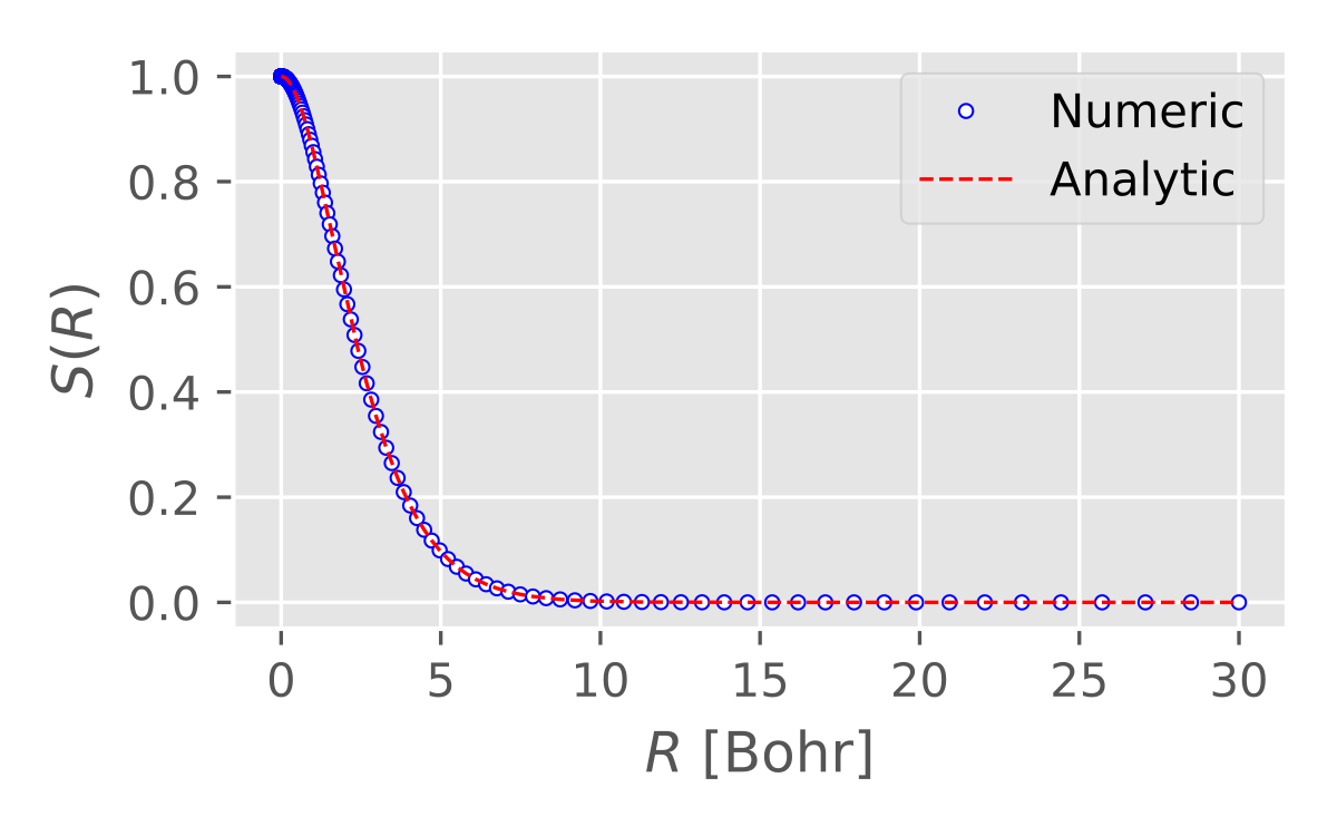
As is well known, the overlap integral of two hydrogen 1s orbitals can be written as
\[\begin{equation} S(R) = e^{-R}\cdot(1 + R + \frac{R^2}{3}) \end{equation}\]Below, we show the comparison of the overlap integral from numerical evaluation and analytic solution.
1
2
3
4
5
6
7
8
9
10
11
12
13
14
15
16
17
18
19
20
21
22
23
24
25
26
27
28
29
30
31
32
33
34
35
36
37
38
39
40
41
42
43
#!/usr/bin/env python

import numpy as np
from pysbt import sbt
from pysbt import GauntTable

N    = 256
rmin = 2.0 / 1024 / 32
rmax = 30
rr   = np.logspace(np.log10(rmin), np.log10(rmax), N, endpoint=True)
f1   = 2*np.exp(-rr)                                # R_{10}(r)
Y10  = 1 / 2 / np.sqrt(np.pi)

ss = sbt(rr)                                        # init SBT
g1 = ss.run(f1, direction=1, norm=True)             # SBT
s1 = ss.run(g1 * g1, direction=-1, norm=False)      # iSBT

sR = 4*np.pi * GauntTable(0, 0, 0, 0, 0, 0) * Y10 * s1

import matplotlib.pyplot as plt
plt.style.use('ggplot')

fig = plt.figure(
  dpi=300,
  figsize=(4, 2.5),
)

ax = plt.subplot()

ax.plot(rr, sR, ls='none', color='b',
        marker='o', ms=3, mew=0.5, mfc='w',
        label='Numeric')
ax.plot(rr, np.exp(-rr) * (1 + rr + rr**2 / 3),
        color='r', lw=0.8, ls='--', label='Analytic')

ax.legend(loc='upper right')

ax.set_xlabel('$R$ [Bohr]', labelpad=5)
ax.set_ylabel('$S(R)$', labelpad=5)

plt.tight_layout()
plt.savefig('s10.svg')
plt.show()