基于Mathematica的三电荷系统运动周期的研究

发布日期: 2022-05-23

文章字数: 325

原始数据

基于Mathematica的三电荷系统运动周期的研究.pdf
Mathematica代码.nb
Mathematica导出数据.xlsx

原始代码

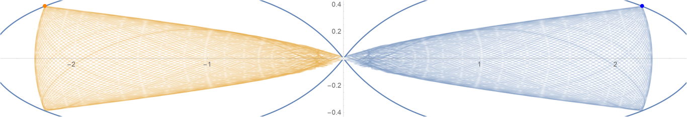
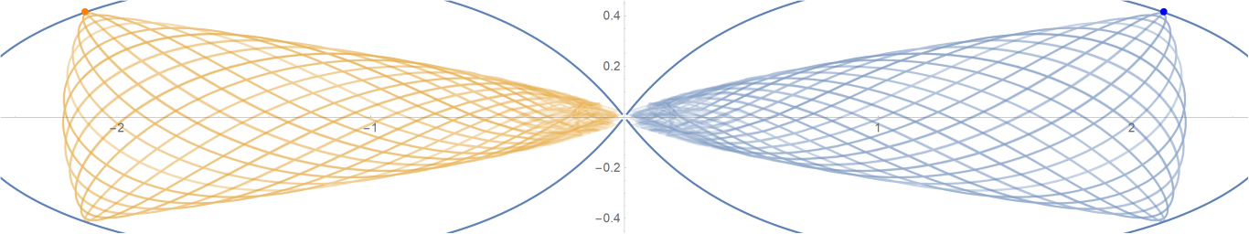
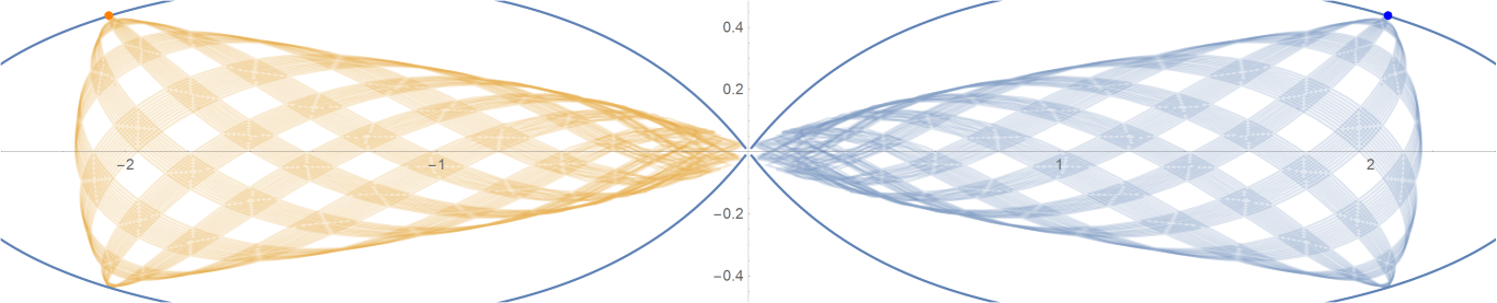
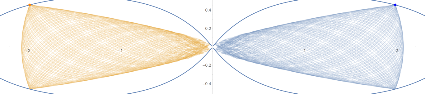
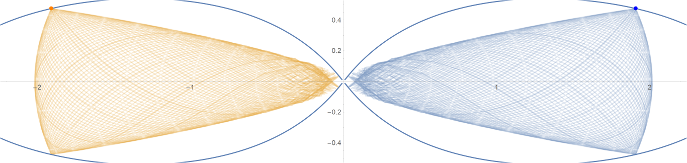
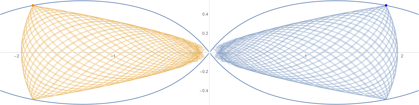
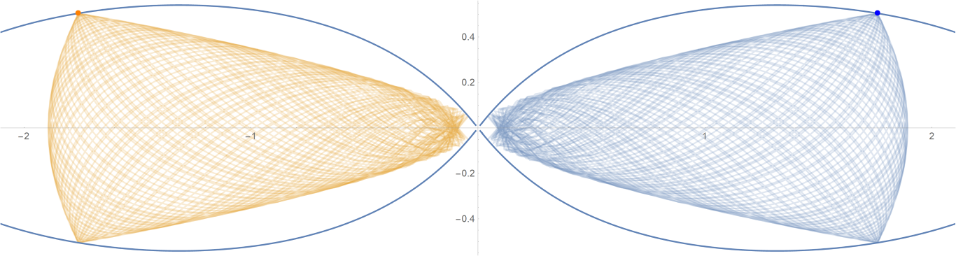
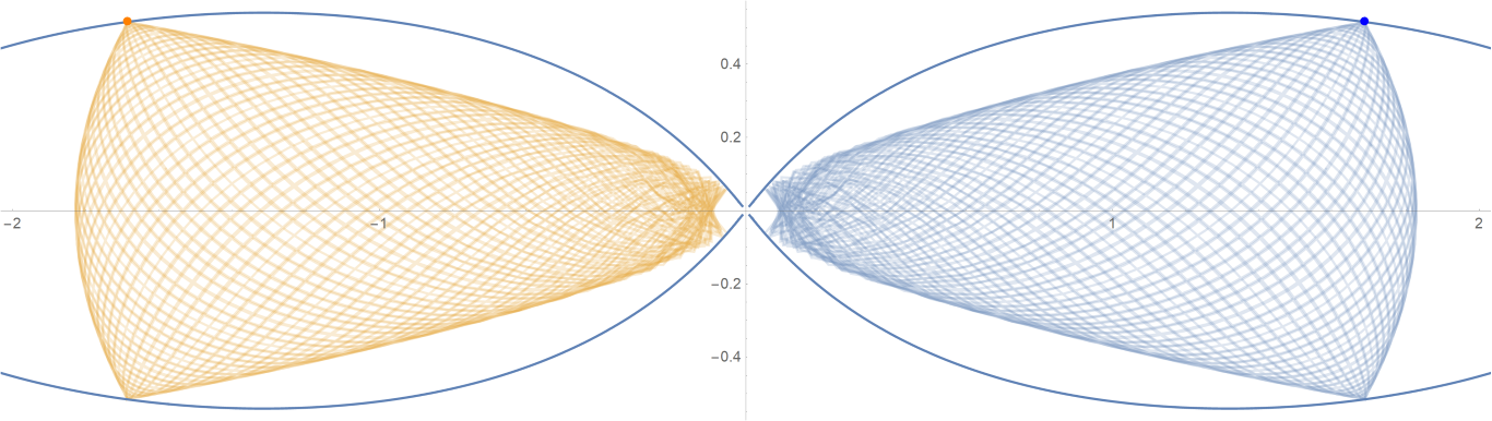
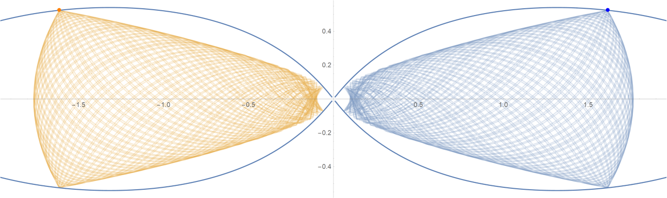
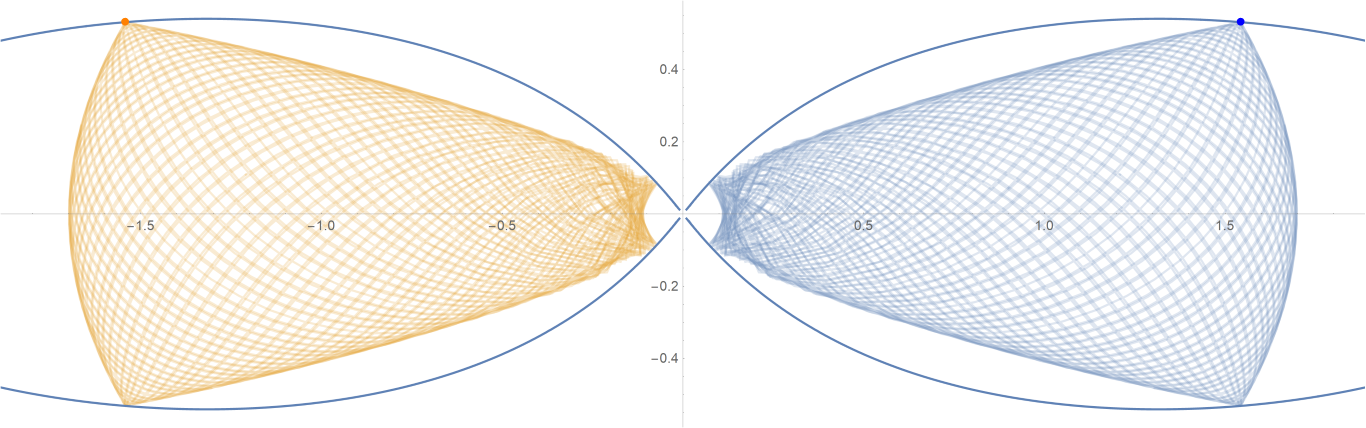
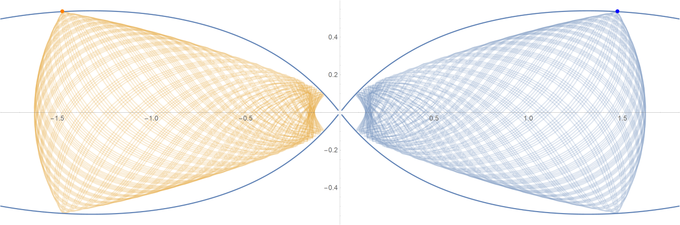
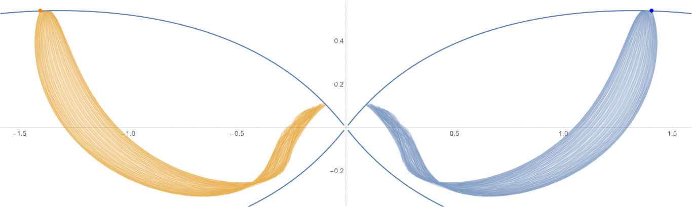
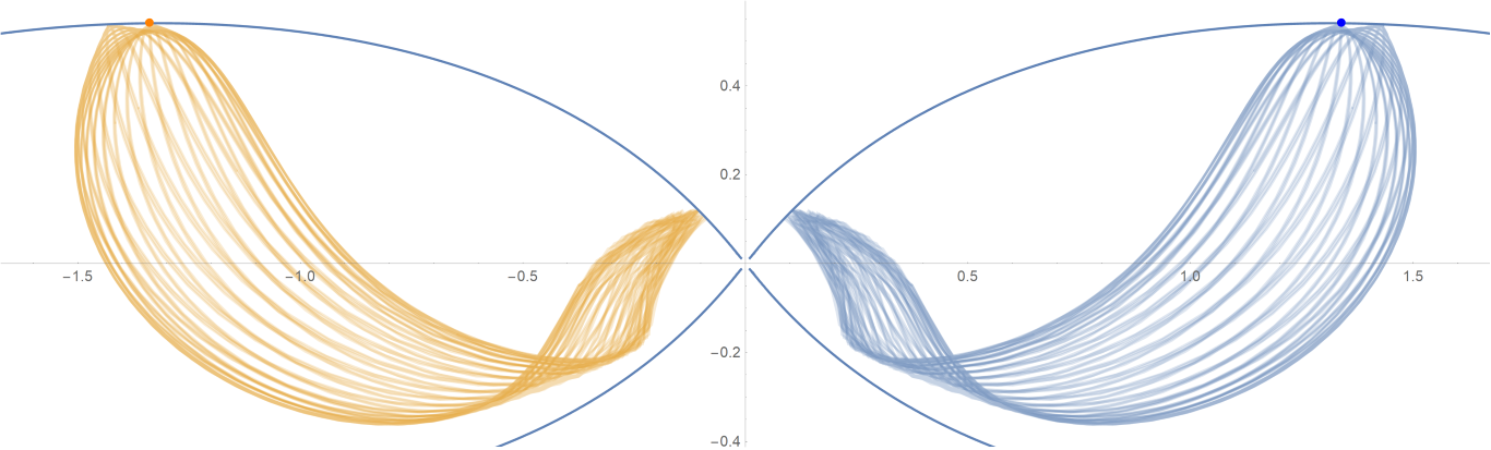
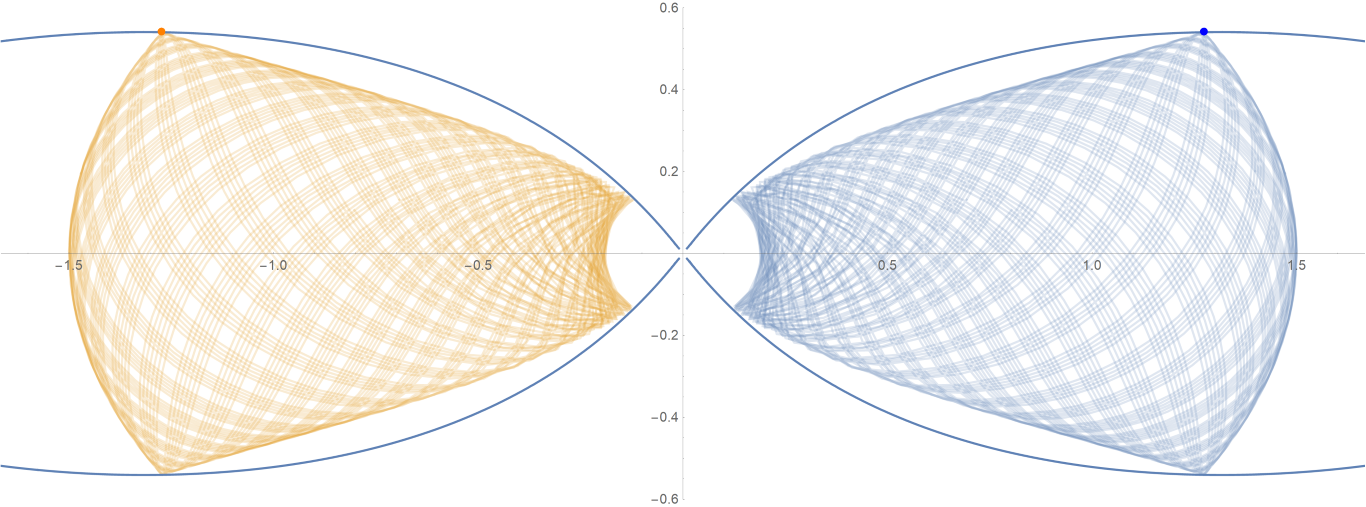
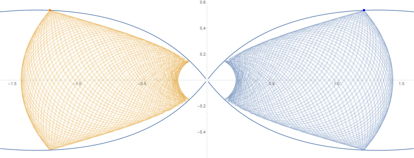
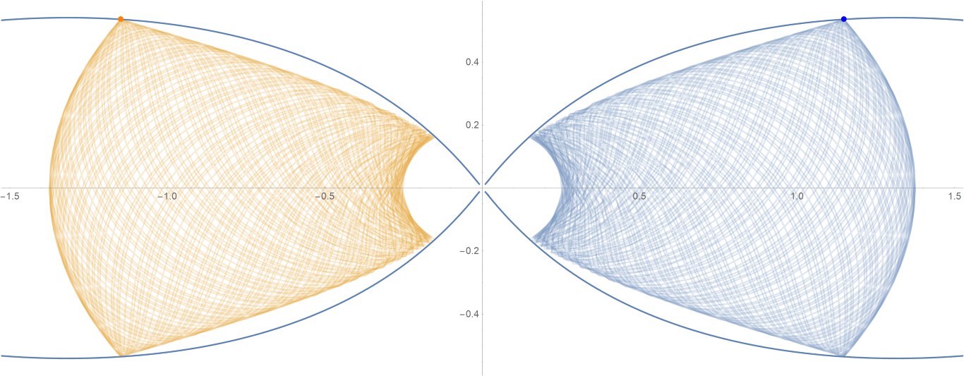
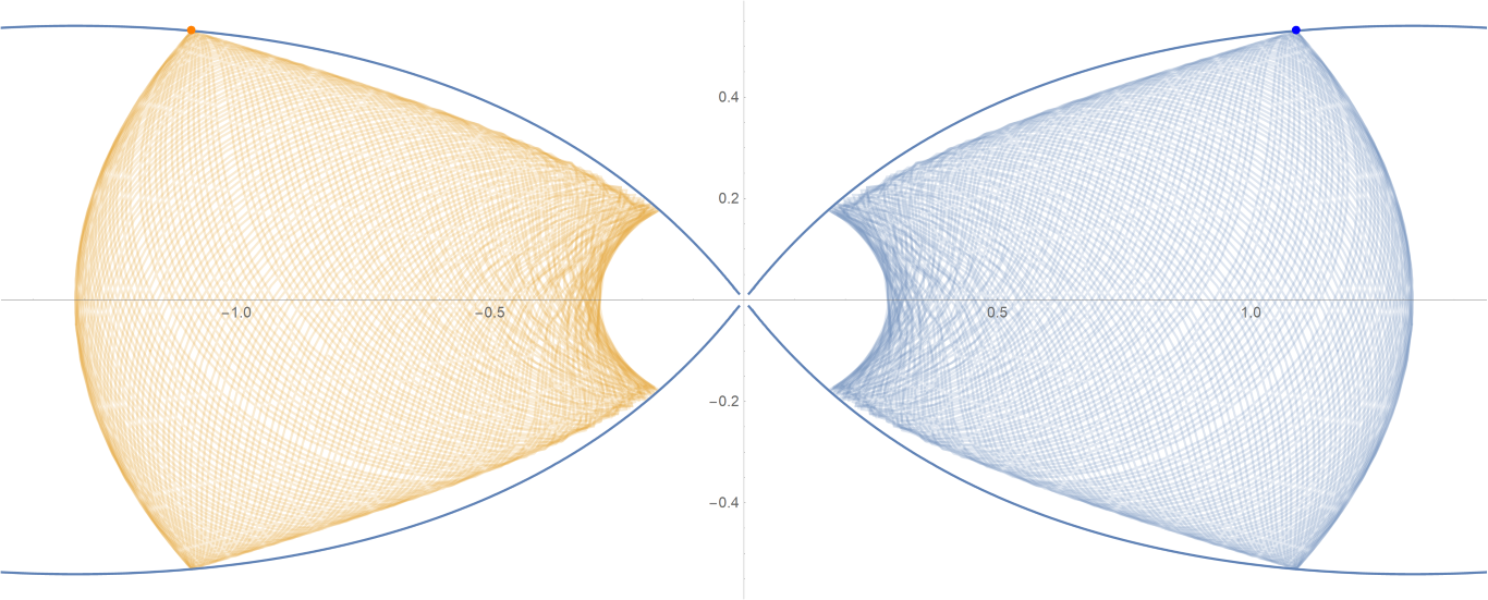
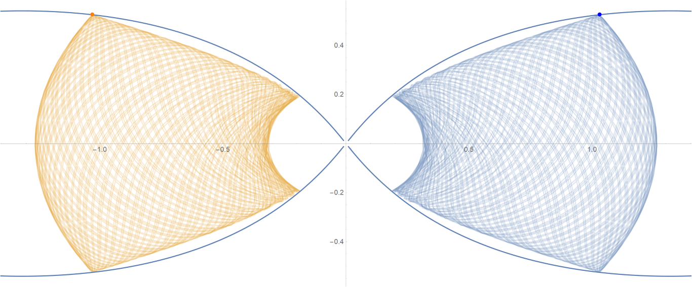
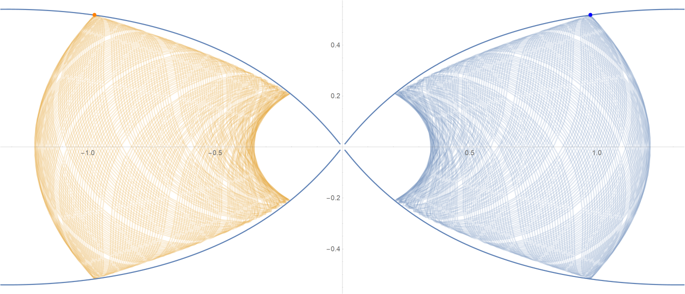
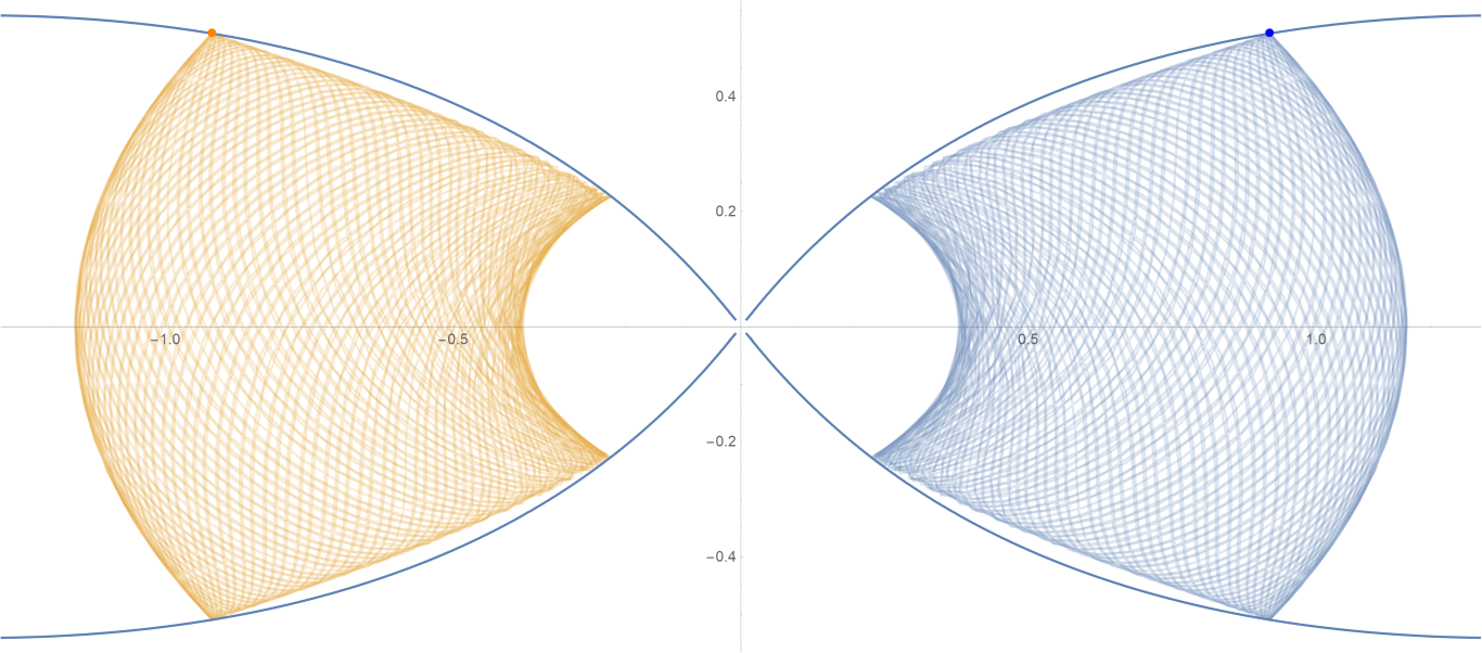
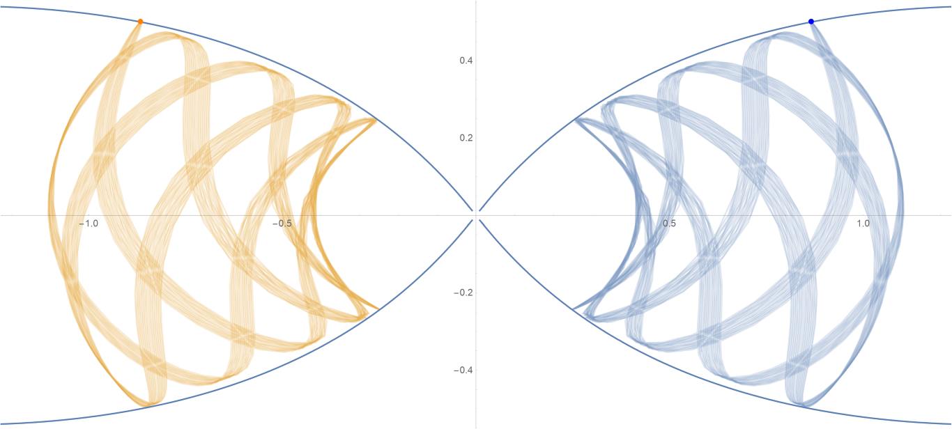
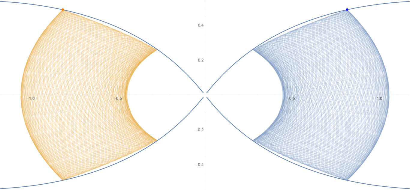
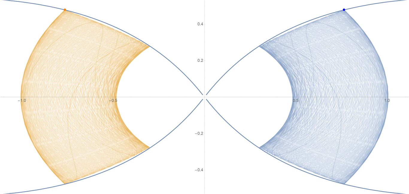
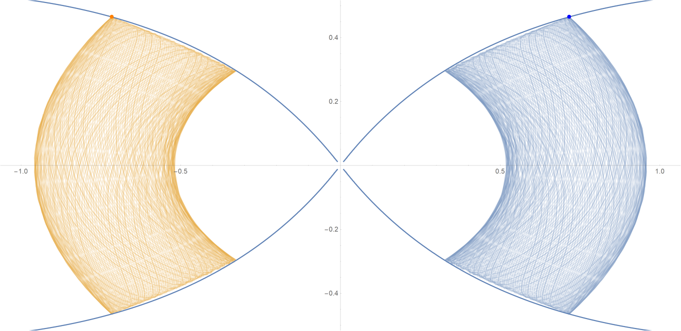
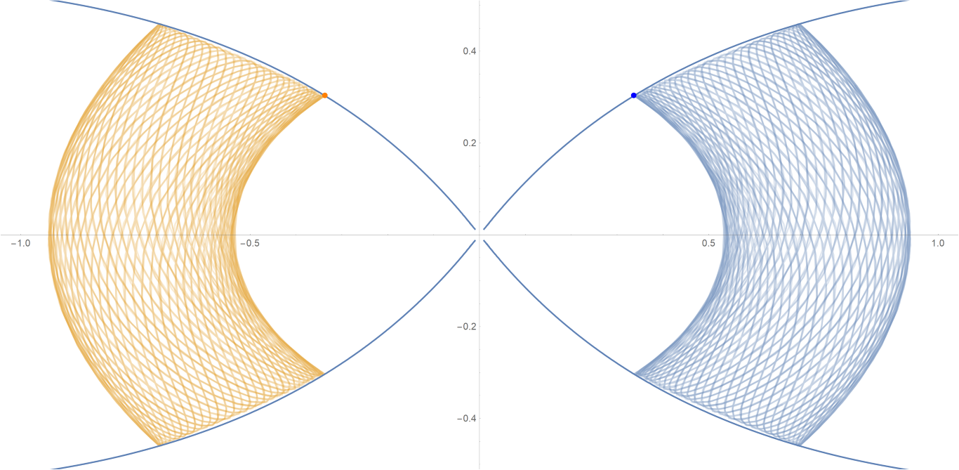
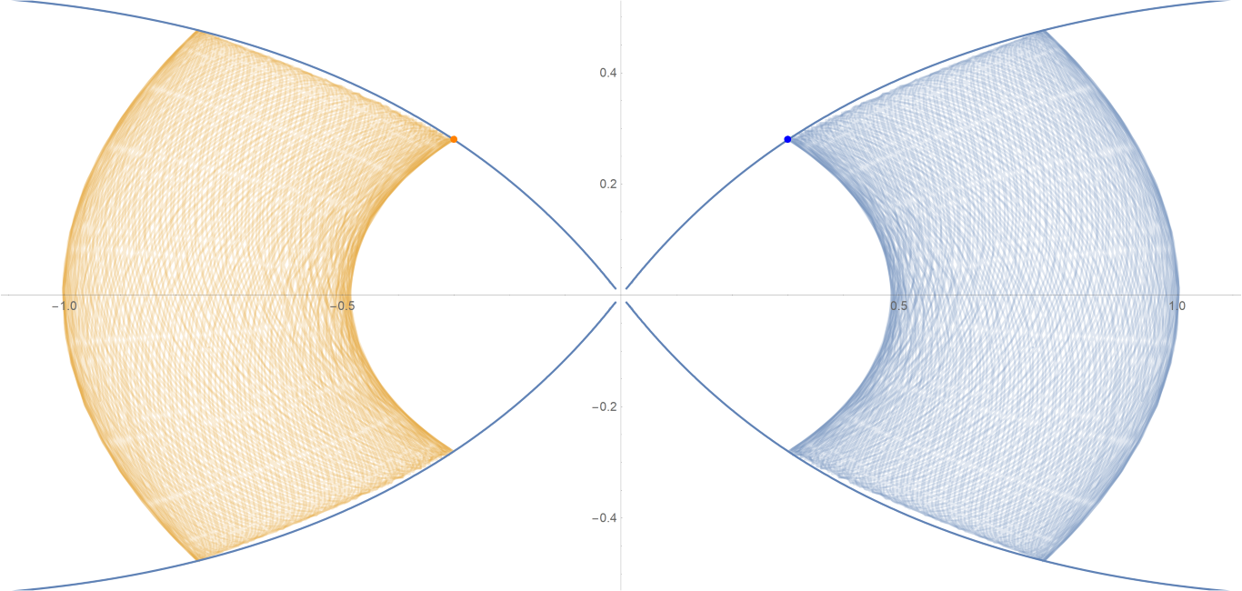
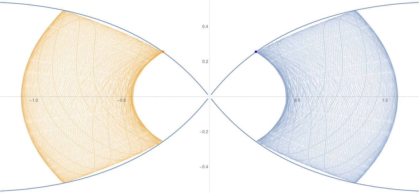
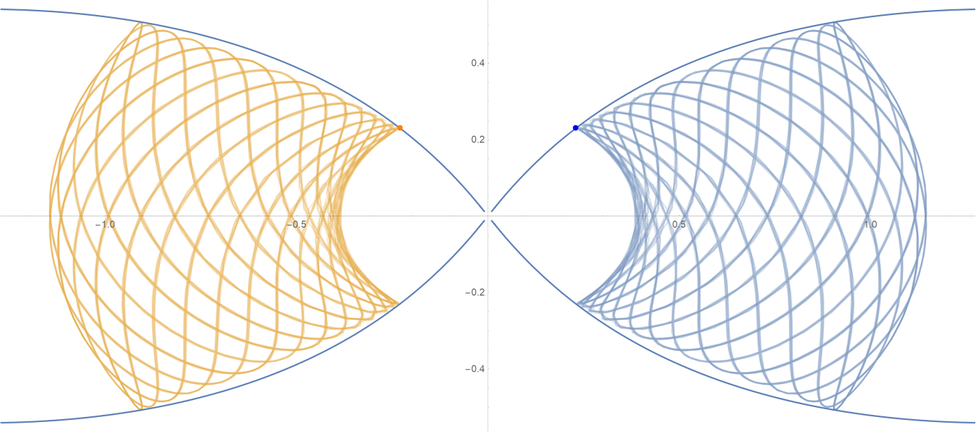
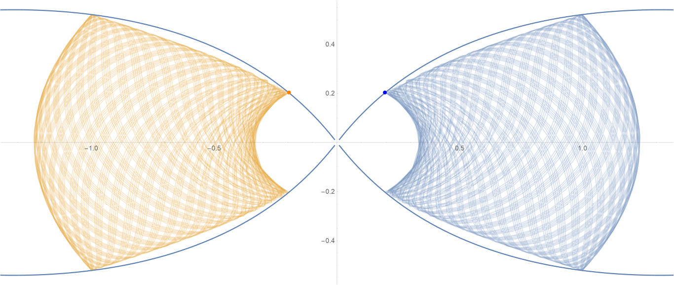
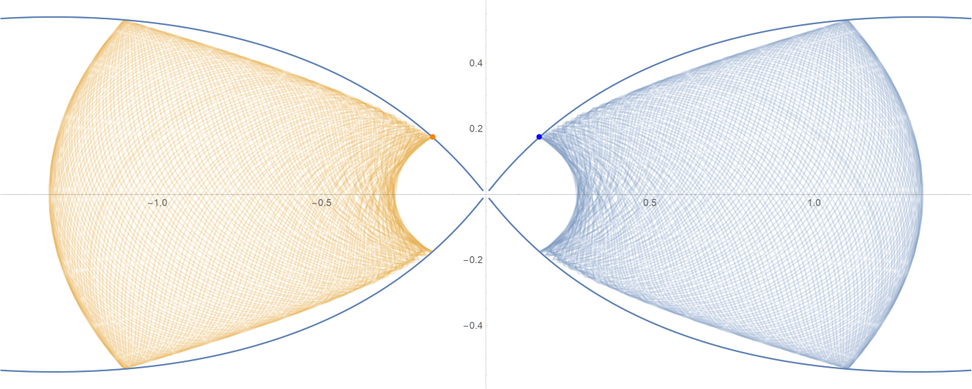
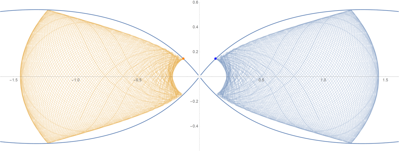
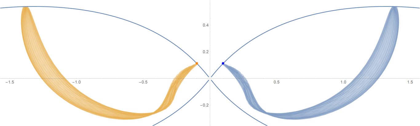
(*Do[{*)tmax = 500; \[Theta]0 = (45*\[Pi])/180; r0 = (
 1/(2 Cos[\[Theta]0]) - 2/Sqrt[
  9 Sin[\[Theta]0]^2 + Cos[\[Theta]0]^2])/-(1/Sqrt[3]); x0 = 
 r0 Cos[\[Theta]0]; y0 = r0 Sin[\[Theta]0]; sol = 
 NDSolve[{(x^\[Prime]\[Prime])[t] == 
    1/(4 x[t]^2) - x[t]/(x[t]^2 + 9 y[t]^2)^(3/2), (
     y^\[Prime]\[Prime])[t] == -((3 y[t])/(x[t]^2 + 9 y[t]^2)^(3/2)), 
   Derivative[1][x][0] == 0, Derivative[1][y][0] == 0, x[0] == x0, 
   y[0] == y0}, {x[t], y[t]}, {t, -0.001, tmax}]; px = 
 x[t] /. Flatten[sol][[1]]; py = y[t] /. Flatten[sol][[2]];
(*Data1=Table[px,{t,0,tmax,0.1}];Export["C:\\Users\\19685\\Desktop\\\
Outx.txt",Data1,"Table"];
Data2=Table[py,{t,0,tmax,0.1}];Export["C:\\Users\\19685\\Desktop\\\
Outy.txt",Data2,"Table"];*)
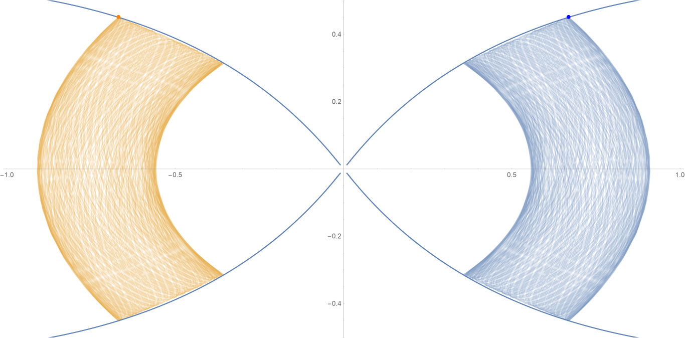
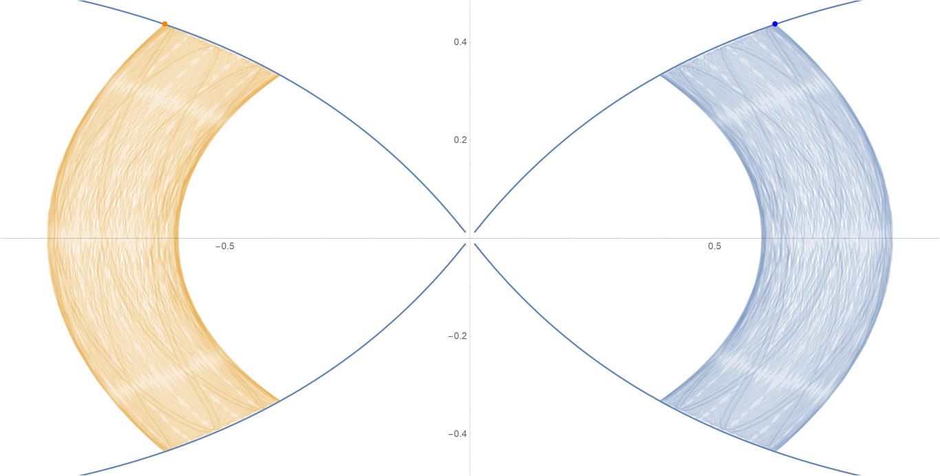
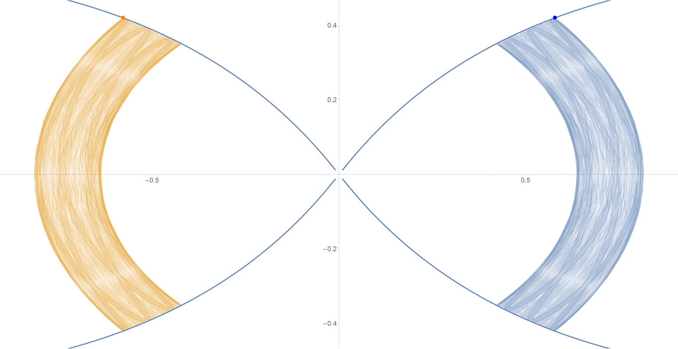
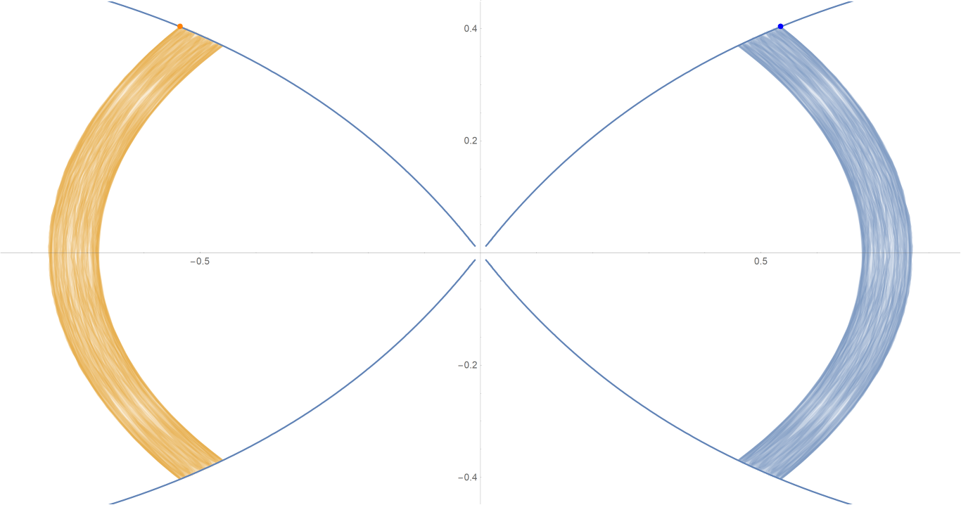
(*Export[{ToString[n]<>".png"},Show[ParametricPlot[{{px,py},{-px,py}},\
{t,-0.001,tmax},PlotStyle\[Rule]{{Opacity[0.2]},{Opacity[0.2]}},\
ImageSize\[Rule]1000],ContourPlot[1/(2Abs[x])-2/Sqrt[x^2+9y^2]\[Equal]\
-(1/Sqrt[3]),{x,-3,3},{y,-1,1},PlotPoints\[Rule]100],Graphics[{Text[\
Style["\[CenterDot]",FontSize\[Rule]50,Blue],{x0,y0}],Text[Style["\
\[CenterDot]",FontSize\[Rule]50,Orange],{-x0,y0}]}]],ImageResolution\
\[Rule]100]},{n,3,50,1}]*)
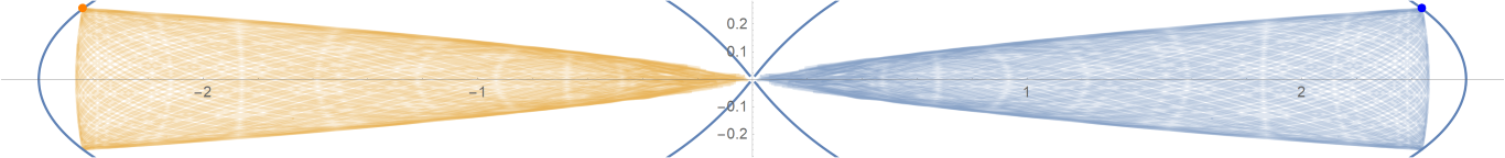
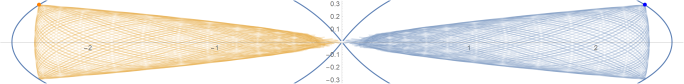
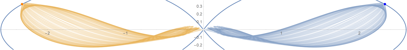
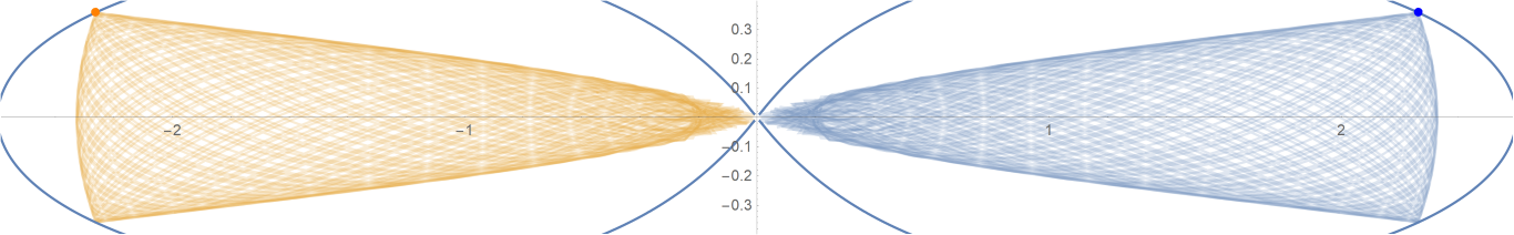
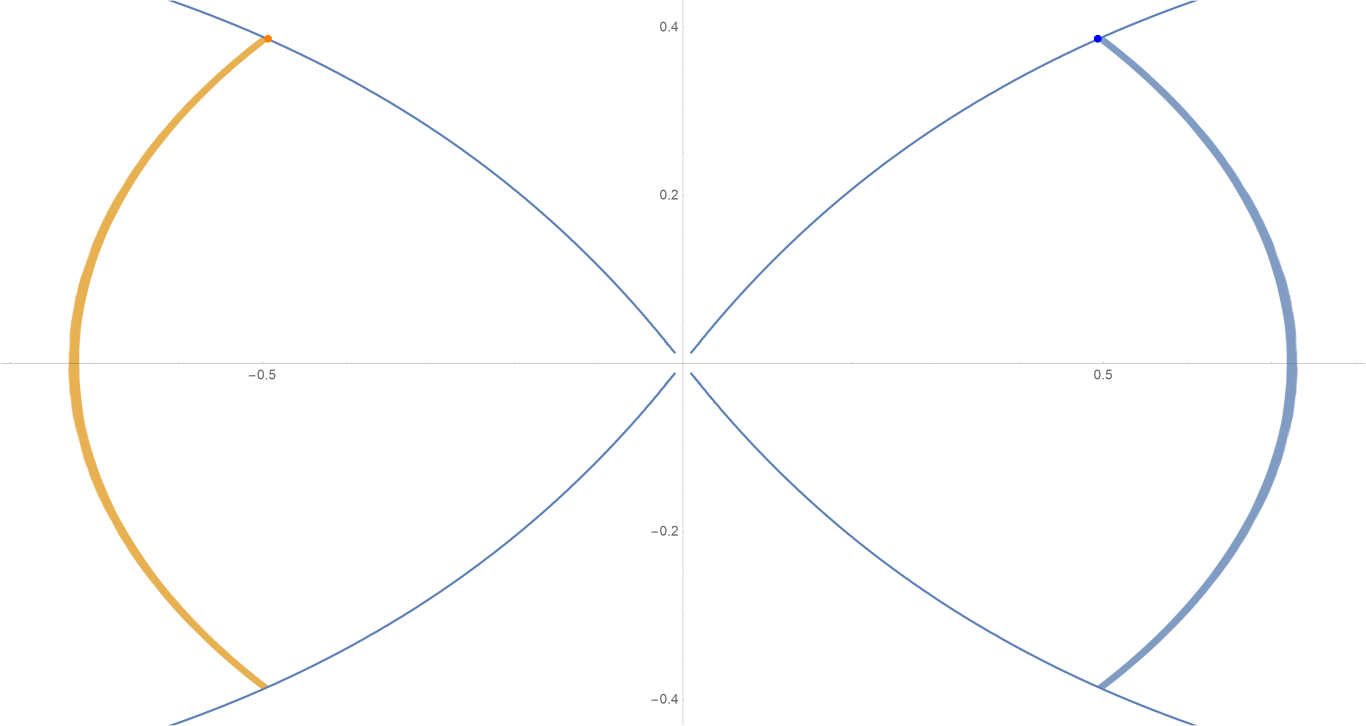
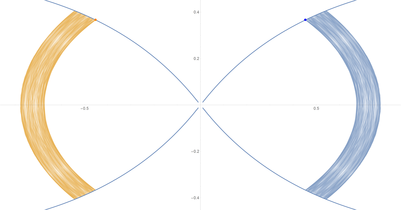
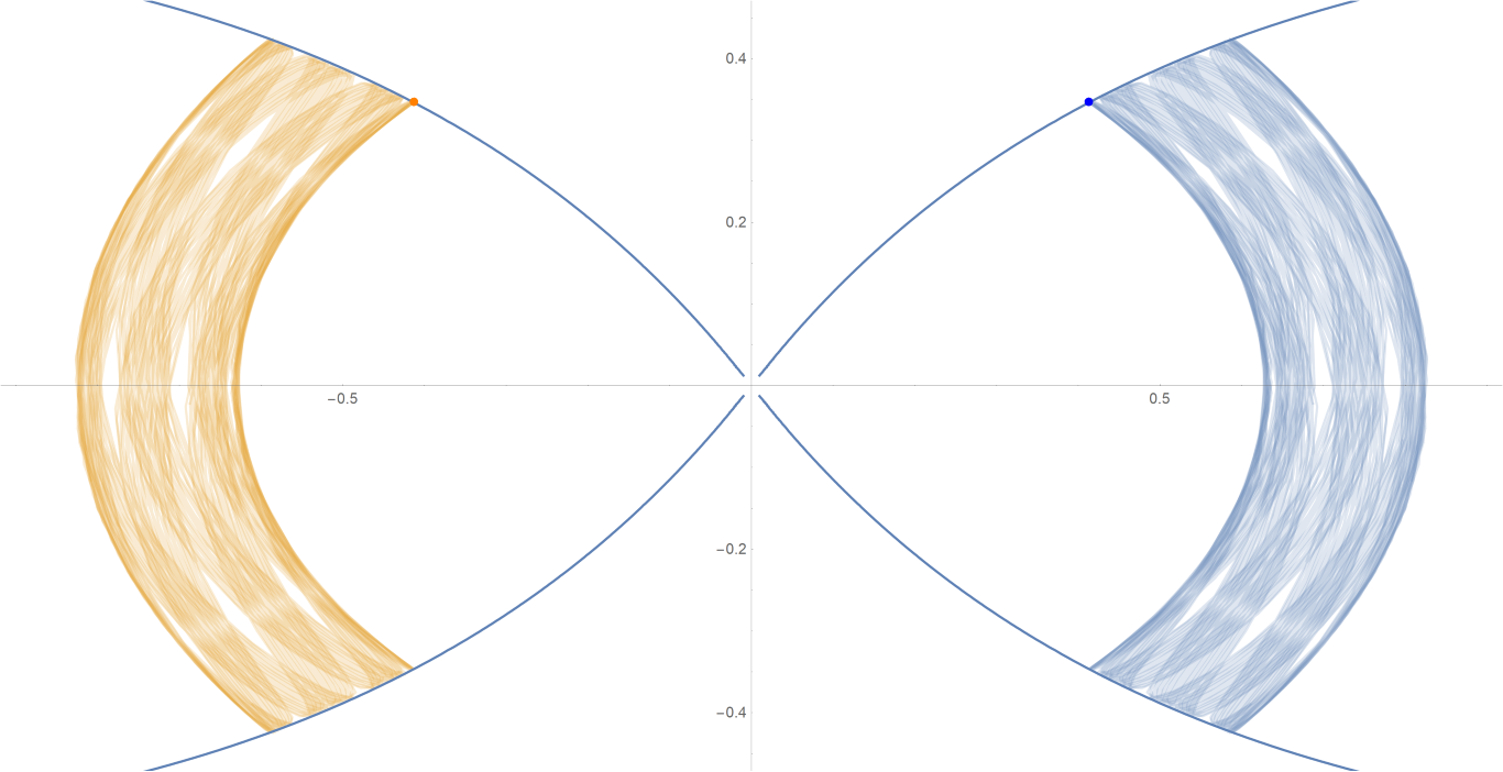
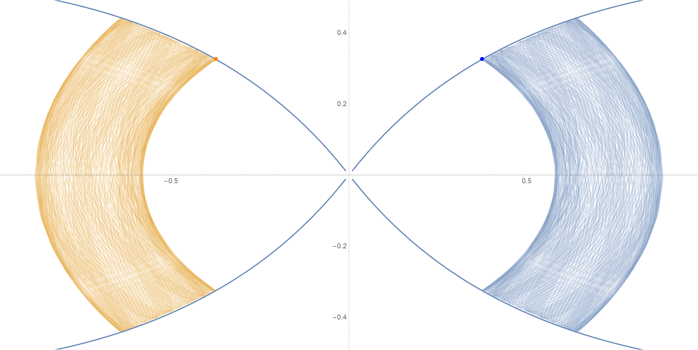
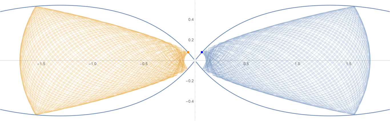
Show[ParametricPlot[{{px, py}, {-px, py}}, {t, -0.001, tmax}, 
  PlotStyle -> {{Opacity[0.75]}, {Opacity[0.75]}}], 
 ContourPlot[
  1/(2 Abs[x]) - 2/Sqrt[x^2 + 9 y^2] == -(1/Sqrt[3]), {x, -3, 
   3}, {y, -1, 1}, PlotPoints -> 100], 
 Graphics[{Text[
    Style["\[CenterDot]", FontSize -> 50, Blue], {x0, y0}], 
   Text[Style["\[CenterDot]", FontSize -> 50, Orange], {-x0, y0}]}]]

数据图片(单位为度数)

Campus